Twitterature: Mining Twitter Data
Hello again, everybody! I’m back this semester as a DH Prototyping Fellow, and together, Alyssa Collins and I are working on a project titled “Twitterature: Methods and Metadata.” Specifically, we’re hoping to develop a simple way of using Twitter data for literary research. The project is still in its early stages, but we’ve been collecting a lot of data and are now beginning to visualize it (I’m particularly interested in the geolocation of tweets, so I’m trying out a few mapping options). In this post, I want to layout our methods for collecting Twitter data.
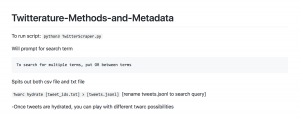
Okay, Alyssa and I have been using a python based Twitter scraping script, which we modified to search Twitter without any time limitations (the official Twitter search function is limited to tweets of the past two weeks). So, to run the Twitter scraping script, I entered the following in my command line: python3 TwitterScraper.py. This command then prompted for the search term and the dates within which I wanted to run my search. For this post, I ran the search term #twitterature (and no, the python scraper has no problem handling hashtags as part of the search query!). After entering the necessary information, the command would create both a txt and a csv file with the results of my search.
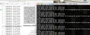
Above: Screen-shot of the python Twitter scraper
Given Twitter’s strict regulations on data usage, the csv files created from my Twitter mining list only a limited amount of information about the tweet, while the txt files just contain the Tweet IDs (a distinct, identifying number that is assigned to each Tweet) that matched my search query.
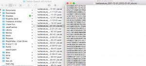
Above: Screen-shot of Tweet IDs
Fortunately, each of these Tweet IDs contains all the data collected from each Tweet; this data is simply encoded. The twarc tools developed by Documenting the Now (DocNow) were instrumental in de-coding this data. That is, DocNow has developed a tool called “Hydrate” that, when applied to a set of Tweet IDs, parses and reveals all of the information associated with each particular Tweet ID. To execute the Hydrate tool, I entered the following into the command line: Twarc hydrate [tweet_ids.txt] > [tweets.jsonl]. In order to avoid confusion, I named each of the jsonl files according to the search term and the dates of the particular query.
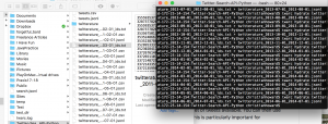
Above: Screen-shot of tweet hydration
For whatever reason, the Twitter scraper occasionally replicated Tweet IDs. As such, I applied the to eliminated redundancies. In particular, I used a twarc tool to “deduplicate” the Tweet IDs. The prompt that I entered into the command line was deduplicate.py [tweets.jsonl] > [deduped_tweets.jsonl].
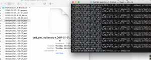
Above: Screen-shot of the deduping process
Once the Tweets were hydrated and deduped, I was able to play with different Twarc possibilities, including geolocation. For the Tweets in which geolocation was available (an option that must be activated by the Twitter user), I was able to output geojson files. Because the geo coordinates associated with Tweets are often not the most exact (sometimes the coordinates are accurate down to a few meters, whereas sometimes the coordinates simply specify the country in which the Tweet originated), I chose to use centroids rather than bounding boxes to indicate Tweet location. In the case where a large area is specified by the geo-coordinates, centroids use the center of the bounding box as approximate location. The command to produce geojson files with centroid-approximated locations was geojson.py [deduped_tweets.jsonl] –centroid > [tweets.geojson].
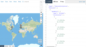
Above: GeoJSON file with bounding boxes
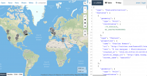
Above: GeoJSON file with centroids
As I mentioned above, for this post I looked specifically at the uses of #twitterature per month from January 2011 through February 2018. Using the method described above, I was able to track the changes in usage over time as well as visualize the locations where #twitterature was tweeted in a given year (and remember, the geolocation data is limited to the tweets in which the user chose to activate geolocation services).

Above: Graph of usage of #twitterature over time
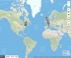
Above: #Twitterature for 2011
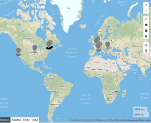
Above: #Twitterature for 2012
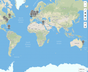
Above: #Twitterature for 2013
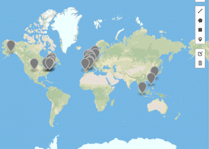
Above: #Twitterature for 2014
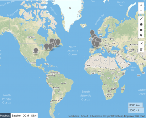
Above: #Twitterature for 2015
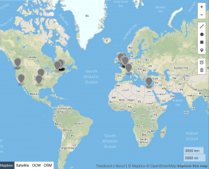
Above: #Twitterature for 2016
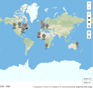
Above: #Twitterature for 2017
As the above data indicates, #twitterature became an increasingly global term between 2011 and 2017, with a noticeable contraction in 2015 (which corresponds to the dip in usage of the hashtag during that same year). It should, of course, be noted that this hashtag is used in primarily English and French speaking countries, and no occurrences of #twitterature are recorded in South America, Russia, China, or other East Asian countries. Despite the prevalence of English in India, #twitterature likewise fails to make an appearance in this country. This dearth may be due to the lack of geospatial data that is available; alternatively, it may indicate that there are other, more popular ways of referring to literature published or disseminated via Twitter in these countries. As we continue working on this project, we’ll look into such alternative references as well as different mapping possibilities to display the data.
So that’s the basic idea! You can download the python scraper (TwitterScraper.py) from our GitHub page: github.com/CHoward345/Twitterature-Methods-and-Metadata. For the DocNow tools, visit: github.com/DocNow/twarc.
We’ll be posting more about the visualization process and our results soon!
And if you want the short version, here you go:
